Examples
The source code of the following code examples can be copied right from this page (to be pasted to YaPyCon, for example), by clicking on the clipboard icon at the top right-hand corner of the source code box.
The icon appears when the mouse pointer hovers over the example’s source code.
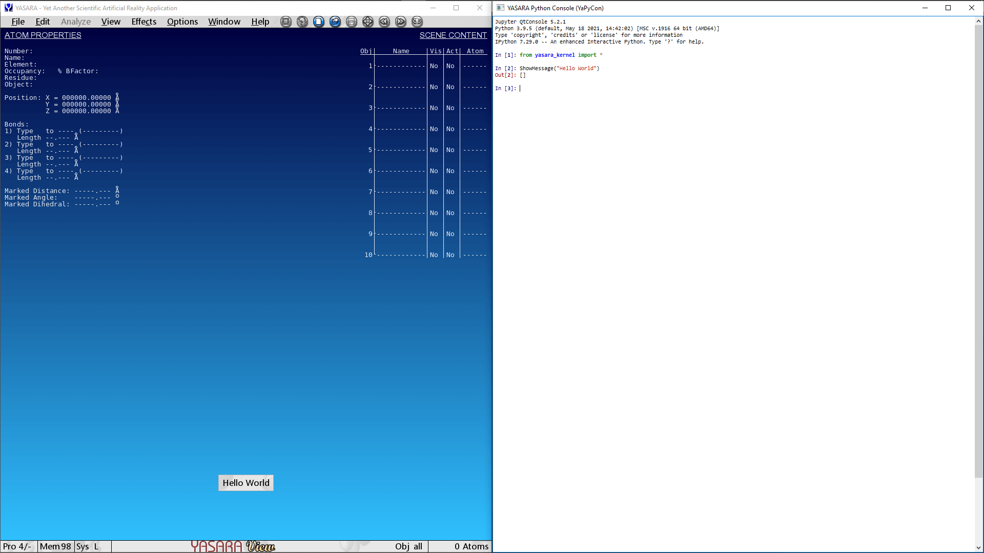
Hello World: YaPyCon Edition
This is perhaps the simplest way to interact with YASARA and get it to display a simple message. This can be achieved as follows:
"""
Displays a message within YASARA.

This code is meant to be executed from
the YaPyCon Python Console.
"""

from yasara_kernel import *
ShowMessage("Hello World")
Accessing YASARA’s pre-defined variables for plugins
Plugins can access a number of predefined variables that are made available to them from the main program and all of them can be accessed from the console.
For example, go ahead and check the owner information that is hard-coded in the software for you. In my case,
these were:
In [3]: owner.familyname
Out[3]: 'Anastasiou'

In [4]: owner.firstname
Out[4]: 'Athanasios'
For another example, let’s check what “stage” our YASARA installation is at. The “stage” defines the availability of certain functionality to YASARA. The “View” stage is the entry level with all of its functionality provided for free.
In [1]: stage
Out[1]: `View`
Obtaining a screenshot
YASARA offers a number of ways by which screenshots can be produced from within the program itself.
These range from a straightforward screenshot of the current state of the user interface, to high resolution renderings (via POV-Ray), to 3D formats such as point clouds, Wavefront objects and STL files for 3D printing.
This example is about the entry level capability of simply saving a screenshot and it also demonstrates some
additional functionality due to YaPyCon.
In the following script, it is assumed that you have started YASARA and went directly into the console. Notice that the
script already loads a sample molecule ("1CRN") to work with but if you already have something loaded in YASARA,
feel free to skip that part.
"""
Takes a screenshot from YASARA and displays it inline
in the Python Console.

This code is meant to be executed from
the YaPyCon Python Console.
"""

from yasara_kernel import *
from matplotlib import pyplot as plt

%matplotlib inline

LoadPDB("1crn", download="latest")
screenshot_image = SavePNG("some_screenshot.png")
plt.imshow(screenshot_image)
If everything has gone well, you are probably looking at something like this:
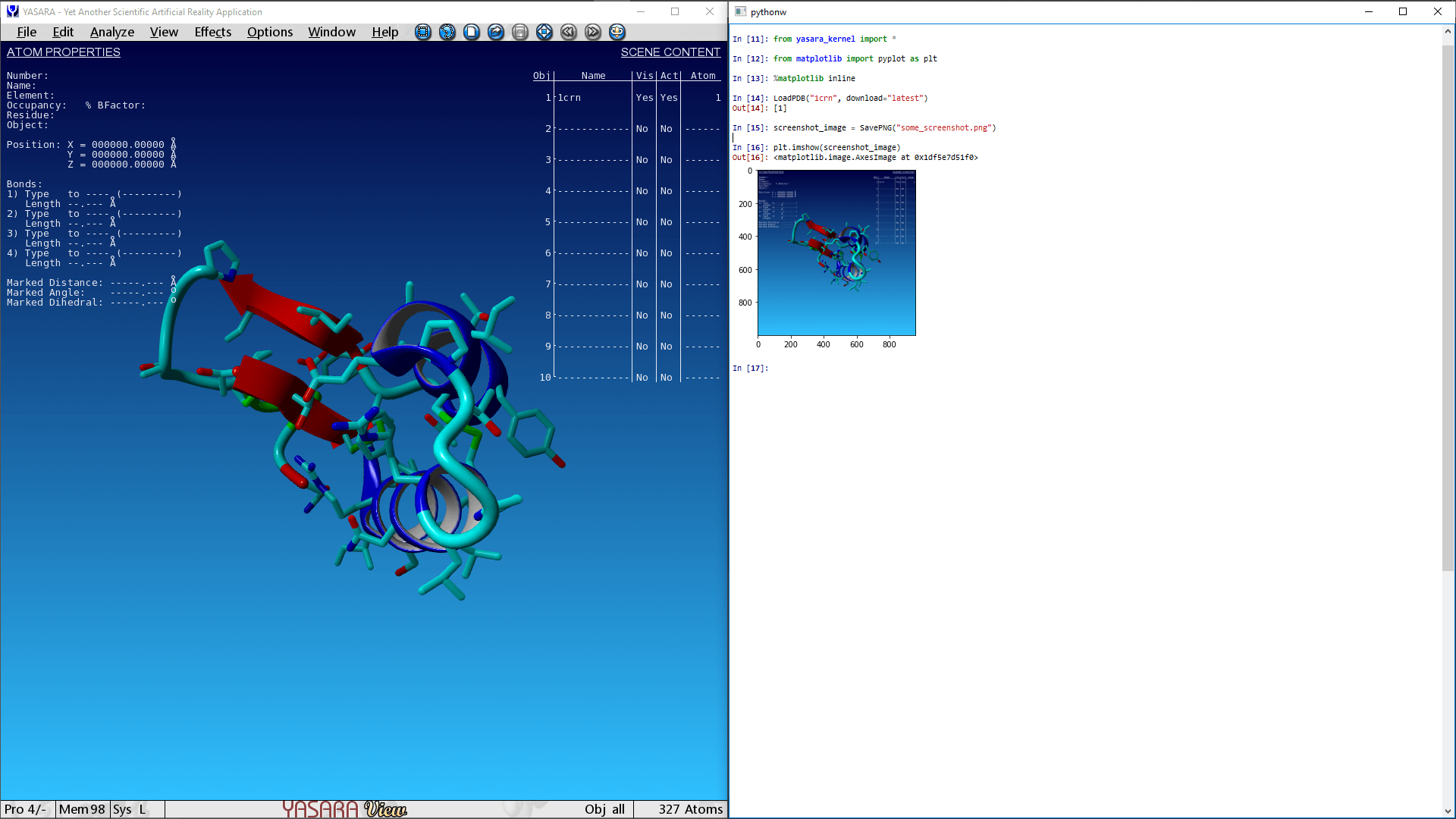
It is worth noting at this point that SavePNG works differently than the standard yasara module, SavePNG
function. Normally, SavePNG() would return the result of the command, but when you load yasara_kernel, the
same command will return a numpy array with the screenshot that was just saved from YASARA (if matplotlib is available
in the currently active Python environment).
This small modification, combined with the
“magic” command
%matplotlib inline, enables the Python console to display the image very conveniently within the console itself.
Creating animated GIFs
This is a plain simple re-creation of the built in demo of creating an animated GIF, but executed entirely in
YaPyCon and standard Python.
"""
Produces an animated GIF, entirely through YASARA,
by rotating and obtaining screenshots of a sample molecule.

This code is meant to be executed from
the YaPyCon Python Console.
"""

from yasara_kernel import *
from matplotlib import pyplot as plt
from matplotlib.animation import FuncAnimation
import os

# Load a sample molecule here
LoadPDB("1crn", download="latest")
# Obtain the first frame from YASARA
frame = SavePNG("frame.png", menu="No")

# Prepare the plot to visualise the frame
fig, ax = plt.subplots()
fig.set_tight_layout(True)

def on_update(i):
    RotateObj(1, y=11.25)
    frame = SavePNG("frame.png", menu="no")
    ax.imshow(frame)
    return [ax, ]

anim = FuncAnimation(fig, on_update, frames=range(0,32), interval=200)
anim.save(os.path.expanduser('~/1crn_rotating.gif'), dpi=92,)
This script will produce the following animated gif:
The resulting GIF from this example (1crn_rotating.gif) is stored in the user’s home directory whatever that might
be depending on the platform.
Exporting data in different formats
When YASARA loads a molecule from one of the standard file formats, it performs a few standard sanity checks 1 on the data about the atoms and (more importantly) the bonds of that molecule.
Fortunately, all of this information is available to plugin developers.
YaPyCon extends the existing functionality with some convenience functions that reshape the way information is
returned from YASARA and enable a much faster lookup.
In this example, one of the smallest molecules available in the PDB (1GCN) is loaded in YASARA and converted to
a graph.
A graph (\(G\)) is a mathematical object composed of a set of nodes (\(V\)) connected via edges (\(E\)). In the context of bio-informatics the nodes of the graph representation of a molecule correspond to the molecule’s atoms and the edges correspond to the molecule’s bonds.
Graph representations are very useful in a number of different applications but in this example we are simply creating a graph and visualising it.
Note
The following code, requires the module networkx to be installed in the activated Python environment.
networkx can be installed from PyPi via a simple:
> pip install networkx
"""
Loads a molecule, creates a graph representation of it,
saves the graphml file to the user's home directory and
uses the kamada-kawai force-directed algorithm to render
the graph representation inline in the YaPyCon Python
console.

This code is meant to be executed from
the YaPyCon Python Console.
"""
from yasara_kernel import *
from matplotlib import pyplot as plt
import os
import networkx

%matplotlib inline

# Load a sample molecule here
LoadPDB("1GCN", download="latest")
# Add hydrogens to pH
AddHydAll()

# Define the format for the atom information to be returned
atom_format = "ATOMNUM, ATOMELEMENT, CHARGE"
# Obtain information about the atoms
molecule_atoms = ListAtom("all", format=atom_format)
# Reformat the returned information to a list of dicts with keys obtained from the format.
molecule_atoms = yapycon_reformat_atominfo_returned(molecule_atoms, format=atom_format, delim=",")
# Obtain information about the covalent bonds
molecule_bonds = ListBond("all", "all", results=4)
# Reformat the returned information to a list of dicts with keys
# the specific attributes for each bond.
molecule_bonds = yapycon_reformat_bondinfo_returned(molecule_bonds, num_of_results=4)

# Build up the graph
g = networkx.Graph()
# Add the nodes
for an_atom in molecule_atoms:
    g.add_node(an_atom["ATOMNUM"], element=an_atom["ATOMELEMENT"], charge=an_atom["CHARGE"])
# Add the edges
for a_bond in molecule_bonds:
    g.add_edge(a_bond["atomnum_sel1"], a_bond["atomnum_sel2"],
               bond_order=a_bond["bond_order"], bond_length=a_bond["bond_length"])

# At this point, we are ready to save or visualise the network.
# Save the file as graphml to the users documents directory
networkx.write_graphml(g, os.path.expanduser("~/yasara_molecule.graphml"))
# Set the atom element as the node's label
node_labels = dict(map(lambda x:(x[0], x[1]["element"]), g.nodes(data=True)))
# Use the built in networkx functionality to visualise the network
fig = plt.figure(figsize=(12,10), dpi=92);
networkx.draw_kamada_kawai(g, with_labels=True, labels=node_labels, ax=plt.gca())
This code snippet saves the network in the file yasara_molecule.graphml in the user’s home directory
(C:\Users\<username> in MS Windows, /home/<username> in Linux) and also uses the Kamada-Kawai force
directed algorithm to provide a simple rendering of the network data.
In this rendering (available below), each node is labeled with the atom’s element:
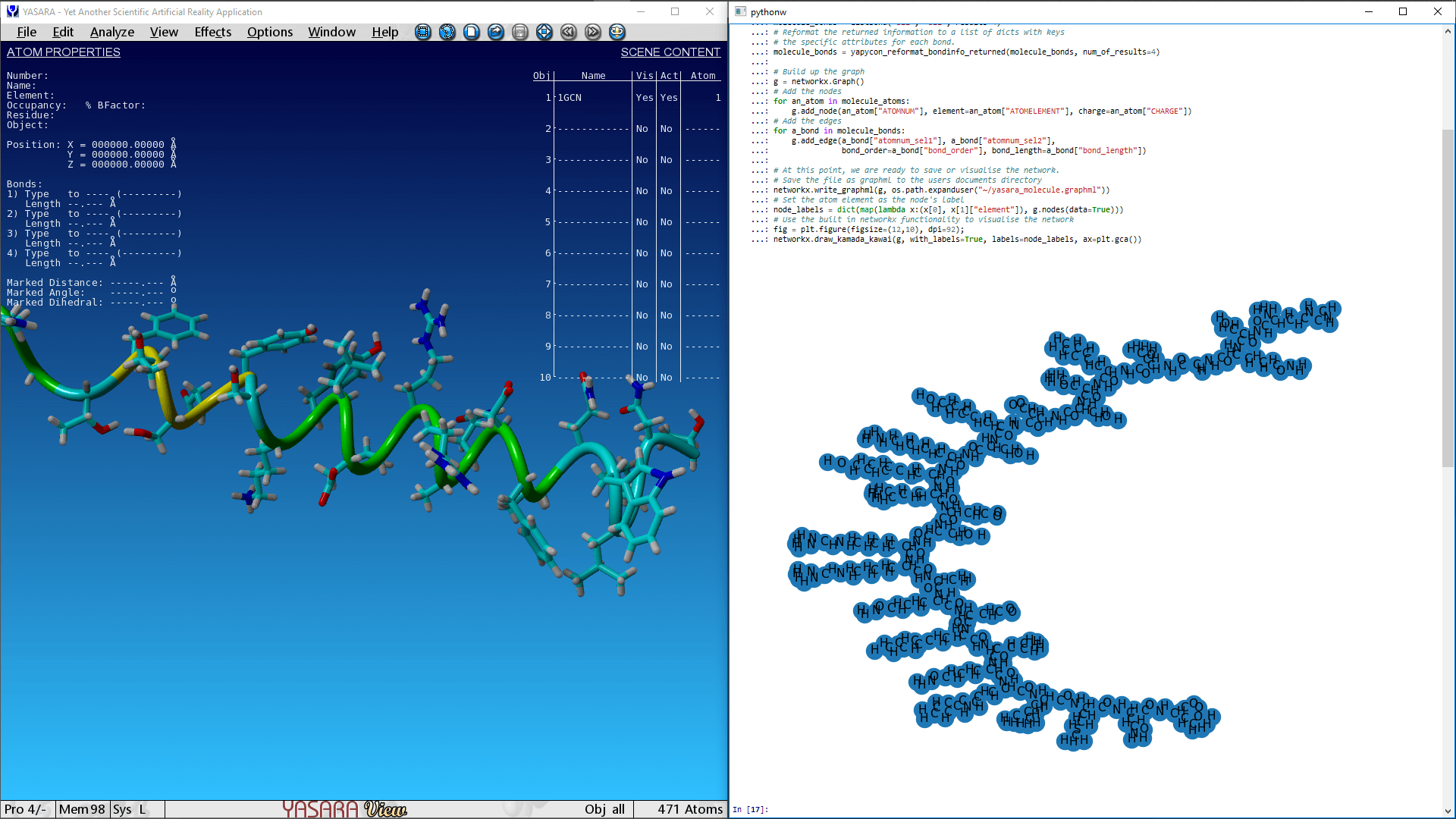
It is worth noting here that the above graph representation includes only the covalent bonds of a molecule.
YASARA does provide functions to “list” (i.e, to retrieve information about) “bonds” and interactions of different types (e.g. hydrogen bonds, hydrophobic interactions, pi-pi interactions and others) that contribute to the tertiary structure of a given molecule but this functionality is not available at the YASARA View stage.
- 1
Sanity checks are applied at different levels and “stages”. The entry level stage, YASARA View, performs 4 standard checks as part of the
LoadPDBcommand but theCleancommand of the YASARA Model stage, performs 39 checks to counteract a variety of known data quality issues.